Written by Keir Johnson
on August 03, 2018

Up your data visualization game with plotly

“What is that?!” is what you’ll hear from your colleagues when you start creating beautiful data visualizations with only a few lines of code. With a little Python code and a package called ‘ploty’, you’ll be the talk of the town. As you can see from the choropleth chart below, a beautifully rendered visualization adds style, flare, and a sense of scientifically-proven-credibility to a data set, in this case, reported Bigfoot (Sasquatch) sightings per U.S. state.

A picture is worth a thousand words

As you have now seen, you can really take things up a notch with data visualization libraries in Python. In this post, we will cover the basics of generating data visualizations using a library called plotly. As with most things, there are a variety of data visualization libraries to choose from, including Matplotlib, Bokeh, and Seaborne. Each library is capable of producing beautiful data visualizations and it’s well worth investing the time to learn how to use them! I am covering plotly simply because, of all the libraries, I have used it the most and find it to be versatile for generating visualizations that are interactive, nice to look at, and are hassle-free for sharing with others via email or the web.

What is plotly?

Let’s take a look at plotly. Plotly offers a suite of open-source tools for producing interactive data visualizations with a focus for the web. Visiting the Python-focused version of plotly’s site will give you a sense of the wide range of visualizations that are possible. Further perusal of the site will reveal a plethora of configuration options for customizing the appearance and interactivity of the charts.

You’ll probably also notice that plotly offers an online platform for hosting and configuring visualizations and dashboards. If you are just creating visualizations for yourself or your team and don’t need to host your visualizations online, there is an option to produce them locally, without using the hosting service. For this use-case, plotly will generate a self-contained HTML file that is interactive and can be viewed in a web-browser, easily shared with others (e.g., as an email attachment), and is generally pretty great-looking right out of the box! This is what I will cover below.

Install plotly

At the time of writing this post, plotly is not included by default in the Anaconda distribution and so you’ll need to install it before referencing plotly in code. If you followed my post from June 8th you will have the conda package manager installed and can install ploty by opening a terminal window and executing the command conda install plotly. If you have never installed a package using conda before, the conda documentation provides helpful instruction.

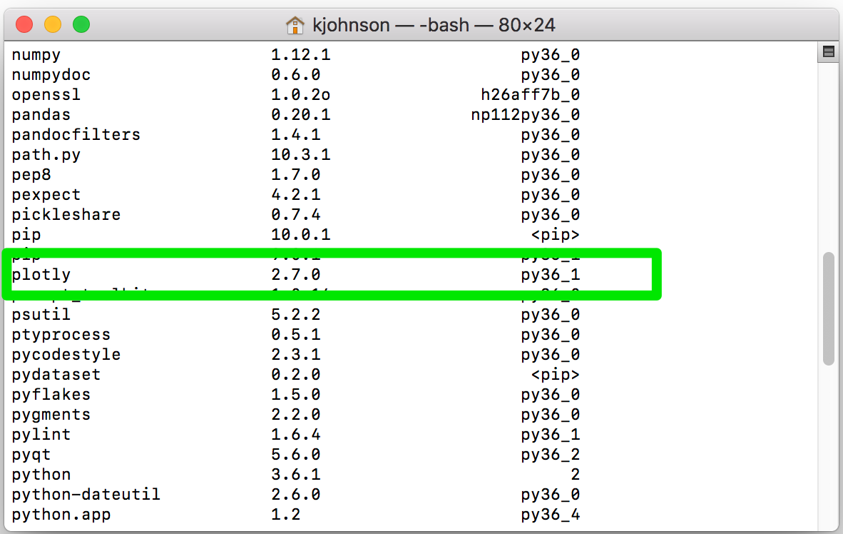
After following the prompts to install plotly using conda, you can verify that it did indeed install successfully by typing conda list and finding plotly in the list of installed packages.

installed packages — Yep, plotly is installed

How to use plotly

Generating a data visualization using plotly can be summarized by the process below:

Import plotly.plotly and plotly.graph_objs (assuming plotly is installed already)
Arrange your data in the required structure according to visualization type (e.g., bar chart, line chart, boxplot, etc.) and store the data in what I will refer to as a ‘data’ object
Configure formatting settings (e.g., chart title, axis titles, legend position, etc.) and store them in a ‘layout’ object
Combine the ‘data’ object and the ‘layout’ object in a ‘figure’ object
Use plotly to generate the visualization from the ‘figure’ object (with appropriate output settings)

In my experience, the most difficult step is arranging the data (step 2) into the structure required for the visualization. That said, in order to use plotly effectively, you should be comfortable working with Python DataFrames and dictionaries because you will use these frequently to prepare the appropriate data structure for a plotly visualization.

Before getting started, a quick word on why we need to import graph_objs (step 1 above). Looking at plotly’s documentation you might notice that some visualizations (e.g., line charts), use the graph_objs object to store data and other parameters for a data visualization while other chart types (e.g., Heatmap with unequal block sizes), do not use graph_objs directly, and instead, a dictionary is all that is needed. What does this mean?

Plotly charts can use graph_objs and python dictionaries somewhat interchangeably. In cases where graph_objs is used, it is simply providing an plotly-specific method or “interface” for configuring your visualization. However, just because graph_objs is used in the documentation, doesn’t mean it is required. For example, exampleTraceGo and exampleTraceDict in the code block below will produce identical line charts. You can see how exampleTraceGo provides some information to the reader about the type of chart being configured (i.e., Scatter), which is nice, and follows a similar format to a dictionary but without single quotes around the keys and without curly braces to construct it. exampleTraceDict follows the old familiar format of a python dictionary which could be more intuitive if you’re used to working with dictionaries.

import plotly.graph_objs as go

# example using graph_objs
exampleTraceGo = go.Scatter(
        x = [1, 2, 3, 7, 8],
        y = [2, 4, 5, 7, 1],
        name = 'example trend data',
        mode = 'lines+markers')

# example using dictionary
exampleTraceDict = {
         'x' : [1, 2, 3, 7, 8],
        'y' : [2, 4, 5, 7, 1],
        'name' : 'example trend data',
        'mode' : 'lines+markers'}

Whether you decide to use graph_objs or a dictionary to construct your data object, the key thing to remember is that both use key-value pairs. The keys represent the available configuration options and values are the parameters you provide as inputs. When in doubt, follow the plotly documentation.

Now, let’s walk through an example.

Example: Life Expectancy Trends

In this example, we will use a life expectancy data set that is available on data.gov to answer the question of how life expectancy has changed over the past 100 years via a data visualization. The data is available for download here. A line chart visualization seems like a good option for time trend data, so let’s give that a try.

Inspecting the data set we see that life expectancy data has been collected by sex and race. Let’s say we are interested in visualizing life expectancy over time for each value of ‘sex’ (male, female, both sexes). We can use pandas to read in the data and then split it into three separate DataFrames, one for each value of ‘sex’ which will translate to three lines on the chart.

import pandas as pd
import plotly as py
import plotly.graph_objs as go

# read in data
df = pd.read_csv('/Users/kjohnson/Downloads/NCHS_-_Death_rates_and_life_expectancy_at_birth.csv')

# split data for each line on the chart
femaleData = df[(df['Sex'] == 'Female') & (df['Race'] == 'All Races')]
maleData = df[(df['Sex'] == 'Male') & (df['Race'] == 'All Races')]
bothData = df[(df['Sex'] == 'Both Sexes') & (df['Race'] == 'All Races')]

Now we can build out the objects needed for the plotly visualization. First, we will create the trace objects, one for each trend line. In this example, the response variable to be plotted on the y-axis of the chart is life expectancy (the ‘Average Life Expectancy (Years)’ column in the data set). Time (years) will be plotted on the x-axis (the ‘Year’ column in the data set). Configuring the x and y variables is achieved by assigning the appropriate column from the appropriate DataFrame to the ‘x’ and ‘y’ keys in the trace objects as seen below.

In addition to configuring the x and y variables, the ‘name’ key is configured so that the trend line name will be displayed in a chart legend. The ‘mode’ key is assigned a value of ‘lines+markers’ which controls the appearance of the line. Last, each trace object is put into data object which will be used by plotly to generate the three trend lines on the chart.

femaleTrace =  go.Scatter(
        x = femaleData['Year'],
        y = femaleData['Average Life Expectancy (Years)'],
        name = 'Females',
        mode = 'lines+markers')

maleTrace = go.Scatter(
        x = maleData['Year'],
        y = maleData['Average Life Expectancy (Years)'],
        name = 'Males',
        mode = 'lines+markers')

bothTrace = go.Scatter(
        x = bothData['Year'],
        y = bothData['Average Life Expectancy (Years)'],
        name = 'Both Sexes',
        mode = 'lines+markers')

data = [femaleTrace, maleTrace, bothTrace]

Next, the layout for the chart can be configured. The layout object is composed of a set of dictionaries. For example the dictionary used to configure the chart title, {'title': 'YEAR'}, is a dictionary within the ‘layout’ dictionary. If you read through some of the examples in plotly’s documentation you will see how the dictionary structure is useful; there are many configuration options available (e.g., line labels, colors, axis formats, etc.) and using a dictionary structure helps keep things organized and human-readable. In our simple example, all we need are a chart tile and titles for the x and y axis as seen below.

layout = {'title': 'Average Life Expectancy (United States 1900-2015)',
          'xaxis': {'title': 'YEAR'},
          'yaxis': {'title': 'AVG. LIFE EXPECTANCY (YRS)'}}

Now that the data object and the layout object are configured we can put everything together and generate the chart. Plotly will generate an HTML file and will also open the chart in a web-browser automatically. Boom! Done.

figure = dict(data = data, layout = layout)

py.offline.plot(figure, filename = 'LifeExpectancyTrend.html')

But wait, there’s more! It’s worth explaining the configuration parameters used in creating the chart. First, we used py.offline because we are producing the chart locally and not connecting to plotly’s hosting service. The HTML file that is generated can be opened in a web-browser and shared with others like any other file while still maintaining it’s interactivity (you can forget the days of sharing screenshots of Excel charts). Pretty awesome! filename is fairly self-explanatory, it is the filename used when plotly creates the HTML file for the chart.

An additional configuration option for the plot() function which I find useful is auto_open = False. I’ll often use a loop to iterate through a set of values and generate a bunch of charts all at once. In this case, I don’t want every chart to open right away and create a gazillion tabs my web-browser and so I will add auto_open = False so that the the HTML files are created but not opened automatically. In our example, if we wanted to create a chart for every combination of sex and race in the life expectancy data set (nine charts total), we use something like the code below. Building in loops and integrating other python tools is where you’ll start to unlock the power of plotly and save yourself a bunch of time compared to creating charts manually.

import pandas as pd
import plotly as py
import plotly.graph_objs as go

df = pd.read_csv('/Users/kjohnson/Downloads/NCHS_-_Death_rates_and_life_expectancy_at_birth.csv')

sexesList = df['Sex'].unique()
racesList = df['Race'].unique()

chartTitle = 'Average Life Expectancy - {0}, {1} -(United States 1900-2015)'

for sex in sexesList:
   
    for race in racesList:
       
        dfTrend = df[(df['Sex'] == sex) & (df['Race'] == race)]
       
        trace = go.Scatter(
                x = dfTrend['Year'],
                y = dfTrend['Average Life Expectancy (Years)'],
                mode = 'lines+markers')
       
        layout = {'title': chartTitle.format(race, sex),
                  'xaxis': {'title': 'YEAR'},
                  'yaxis': {'title': 'AVG. LIFE EXPECTANCY (YRS)'}}
       
        figure = dict(data = [trace], layout = layout)
       
        filename = 'LifeExpectancy_{0}_{1}.html'.format(race, sex)
       
        py.offline.plot(figure, filename = filename, auto_open = False)

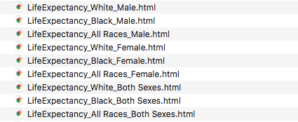
After running the code above and inspecting my working directory, I see that a chart was created for each combination of race and sex.

life expectancy charts — Life expectancy charts ready to go

As I mentioned earlier, plotly is built for the web. To help you display the plotly charts online, the plot() function contains an output type parameter that tells plotly to generate the raw HTML and JavaScript code needed to display the chart in a web-browser. This code can then be embedded directly into a website (btw, that’s how the charts on this page are set up!). Adding output_type = 'div' as seen below will do the trick.

chartSourceCode = py.offline.plot(figure, output_type = 'div', filename = str(filename))

The downside of using output_type = 'div' is that the output is a big, ugly block of code. To avoid this, you can add include_plotlyjs = False so that the minimum amount of HTML and JavaScript is generated. This option, however, will leave you with a block of code that does not display correctly in a web-browser. To get things working again you need to include a reference to plotly’s JavaScript by adding the following line of code at the top of the plotly code block <script src="https://cdn.plot.ly/plotly-latest.min.js"></script>. And now, the chart is interactive again!

chartSourceCode = py.offline.plot(figure, output_type = 'div', include_plotlyjs = False, filename = str(filename))

<!-- plotly's JS reference -->
<script src="https://cdn.plot.ly/plotly-latest.min.js"></script>

<!-- source code generated from using 'output_type = 'div'' -->
<div id="d60f1665-b0c1-4a49-8165-bed388851d45" style="height: 100%; width: 100%;" class="plotly-graph-div"></div><script type="text/javascript">window.PLOTLYENV=window.PLOTLYENV || {};window.PLOTLYENV.BASE_URL="https://plot.ly";Plotly.newPlot("d60f1665-b0c1-4a49-8165-bed388851d45", [{"type": "scatter", "x": [2015, 2014, 2013, 2012, 2011, 2010, 2009, 2008, 2007, 2006, 2005, 2004, 2003, 2002, 2001, 2000, 1999, 1998, 1997, 1996, 1995, 1994, 1993, 1992, 1991, 1990, 1989, 1988, 1987, 1986, 1985, 1984, 1983, 1982, 1981, 1980, 1979, 1978, 1977, 1976, 1975, 1974, 1973, 1972, 1971, 1970, 1969, 1968, 1967, 1966, 1965, 1964, 1963, 1962, 1961, 1960, 1959, 1958, 1957, 1956, 1955, 1954, 1953, 1952, 1951, 1950, 1949, 1948, 1947, 1946, 1945, 1944, 1943, 1942, 1941, 1940, 1939, 1938, 1937, 1936, 1935, 1934, 1933, 1932, 1931, 1930, 1929, 1928, 1927, 1926, 1925, 1924, 1923, 1922, 1921, 1920, 1919, 1918, 1917, 1916, 1915, 1914, 1913, 1912, 1911, 1910, 1909, 1908, 1907, 1906, 1905, 1904, 1903, 1902, 1901, 1900], "y": [null, 81.3, 81.2, 81.2, 81.1, 81.0, 80.9, 80.6, 80.6, 80.3, 80.1, 80.1, 79.7, 79.6, 79.5, 79.7, 79.4, 79.5, 79.4, 79.1, 78.9, 79.0, 78.8, 79.1, 78.9, 78.8, 78.5, 78.3, 78.3, 78.2, 78.2, 78.2, 78.1, 78.1, 77.8, 77.4, 77.8, 77.3, 77.2, 76.8, 76.6, 75.9, 75.3, 75.1, 75.0, 74.7, 74.4, 74.1, 74.3, 73.9, 73.8, 73.7, 73.4, 73.5, 73.6, 73.1, 73.2, 72.9, 72.7, 72.9, 72.8, 72.8, 72.0, 71.6, 71.4, 71.1, 70.7, 69.9, 69.7, 69.4, 67.9, 66.8, 64.4, 67.9, 66.8, 65.2, 65.4, 65.3, 62.4, 60.6, 63.9, 63.3, 65.1, 63.5, 63.1, 61.6, 58.7, 58.3, 62.1, 58.0, 60.6, 61.5, 58.5, 61.0, 61.8, 54.6, 56.0, 42.2, 54.0, 54.3, 56.8, 56.8, 55.0, 55.9, 54.4, 51.8, 53.8, 52.8, 49.9, 50.8, 50.2, 49.1, 52.0, 53.4, 50.6, 48.3], "name": "Females", "mode": "lines+markers"}, {"type": "scatter", "x": [2015, 2014, 2013, 2012, 2011, 2010, 2009, 2008, 2007, 2006, 2005, 2004, 2003, 2002, 2001, 2000, 1999, 1998, 1997, 1996, 1995, 1994, 1993, 1992, 1991, 1990, 1989, 1988, 1987, 1986, 1985, 1984, 1983, 1982, 1981, 1980, 1979, 1978, 1977, 1976, 1975, 1974, 1973, 1972, 1971, 1970, 1969, 1968, 1967, 1966, 1965, 1964, 1963, 1962, 1961, 1960, 1959, 1958, 1957, 1956, 1955, 1954, 1953, 1952, 1951, 1950, 1949, 1948, 1947, 1946, 1945, 1944, 1943, 1942, 1941, 1940, 1939, 1938, 1937, 1936, 1935, 1934, 1933, 1932, 1931, 1930, 1929, 1928, 1927, 1926, 1925, 1924, 1923, 1922, 1921, 1920, 1919, 1918, 1917, 1916, 1915, 1914, 1913, 1912, 1911, 1910, 1909, 1908, 1907, 1906, 1905, 1904, 1903, 1902, 1901, 1900], "y": [null, 76.5, 76.4, 76.4, 76.3, 76.2, 76.0, 75.6, 75.5, 75.2, 75.0, 75.0, 74.5, 74.4, 74.3, 74.3, 73.9, 73.8, 73.6, 73.1, 72.5, 72.4, 72.2, 72.3, 72.0, 71.8, 71.7, 71.4, 71.4, 71.2, 71.1, 71.1, 71.0, 70.8, 70.4, 70.0, 70.0, 69.6, 69.5, 69.1, 68.8, 68.2, 67.6, 67.4, 67.4, 67.1, 66.8, 66.6, 67.0, 66.7, 66.8, 66.8, 66.6, 66.9, 67.1, 66.6, 66.8, 66.6, 66.4, 66.7, 66.7, 66.7, 66.0, 65.8, 65.6, 65.6, 65.2, 64.6, 64.4, 64.4, 63.6, 63.6, 62.4, 64.7, 63.1, 60.8, 62.1, 61.9, 58.0, 56.6, 59.9, 59.3, 61.7, 61.0, 59.4, 58.1, 55.8, 55.6, 59.0, 55.5, 57.6, 58.1, 56.1, 58.4, 60.0, 53.6, 53.5, 36.6, 48.4, 49.6, 52.5, 52.0, 50.3, 51.5, 50.9, 48.4, 50.5, 49.5, 45.6, 46.9, 47.3, 46.2, 49.1, 49.8, 47.6, 46.3], "name": "Males", "mode": "lines+markers"}, {"type": "scatter", "x": [2015, 2014, 2013, 2012, 2011, 2010, 2009, 2008, 2007, 2006, 2005, 2004, 2003, 2002, 2001, 2000, 1999, 1998, 1997, 1996, 1995, 1994, 1993, 1992, 1991, 1990, 1989, 1988, 1987, 1986, 1985, 1984, 1983, 1982, 1981, 1980, 1979, 1978, 1977, 1976, 1975, 1974, 1973, 1972, 1971, 1970, 1969, 1968, 1967, 1966, 1965, 1964, 1963, 1962, 1961, 1960, 1959, 1958, 1957, 1956, 1955, 1954, 1953, 1952, 1951, 1950, 1949, 1948, 1947, 1946, 1945, 1944, 1943, 1942, 1941, 1940, 1939, 1938, 1937, 1936, 1935, 1934, 1933, 1932, 1931, 1930, 1929, 1928, 1927, 1926, 1925, 1924, 1923, 1922, 1921, 1920, 1919, 1918, 1917, 1916, 1915, 1914, 1913, 1912, 1911, 1910, 1909, 1908, 1907, 1906, 1905, 1904, 1903, 1902, 1901, 1900], "y": [null, 78.9, 78.8, 78.8, 78.7, 78.7, 78.5, 78.2, 78.1, 77.8, 77.6, 77.5, 77.6, 77.0, 77.0, 76.8, 76.7, 76.7, 76.5, 76.1, 75.8, 75.7, 75.5, 75.8, 75.5, 75.4, 75.1, 74.9, 74.9, 74.7, 74.7, 74.7, 74.6, 74.5, 74.1, 73.7, 73.9, 73.5, 73.3, 72.9, 72.6, 72.0, 71.4, 71.2, 71.1, 70.8, 70.5, 70.2, 70.5, 70.2, 70.2, 70.2, 69.9, 70.1, 70.2, 69.7, 69.9, 69.6, 69.5, 69.7, 69.6, 69.6, 68.8, 68.6, 68.4, 68.2, 68.0, 67.2, 66.8, 66.7, 65.9, 65.2, 63.3, 66.2, 64.8, 62.9, 63.7, 63.5, 60.0, 58.5, 61.7, 61.1, 63.3, 62.1, 61.1, 59.7, 57.1, 56.8, 60.4, 56.7, 59.0, 59.7, 57.2, 59.6, 60.8, 54.1, 54.7, 39.1, 50.9, 51.7, 54.5, 54.2, 52.5, 53.5, 52.6, 50.0, 52.1, 51.1, 47.6, 48.7, 48.7, 47.6, 50.5, 51.5, 49.1, 47.3], "name": "Both Sexes", "mode": "lines+markers"}], {"title": "Average Life Expectancy - White, Male -(United States 1900-2015)", "xaxis": {"title": "YEAR"}, "yaxis": {"title": "AVG. LIFE EXPECTANCY (YRS)"}}, {"showLink": true, "linkText": "Export to plot.ly"})</script>

If you want to try generating the Bigfoot sightings chart seen at the top of this post, you can follow the code below. I cleaned up the data a bit after copying it from the website (data cleansing is an almost-always necessary task) and saved as a .CSV file locally before creating the plotly chart. The links below will serve as useful references:

Geographic Database of Bigfoot/Sasquatch Sightings and Reports

Plotly Choropleth Maps

import plotly as py

df = pd.read_csv('sasquatch.csv', sep = ',')
df['State code'] = df['State code'].str.upper()

for col in df.columns:
    df[col] = df[col].astype(str)

scl = [[0.0, 'rgb(242,240,247)'],[0.2, 'rgb(218,218,235)'],[0.4, 'rgb(188,189,220)'],\
            [0.6, 'rgb(158,154,200)'],[0.8, 'rgb(117,107,177)'],[1.0, 'rgb(84,39,143)']]

df['text'] = df['State'] + '<br>' +\
            'Most Recent Sighting: ' + df['Most Recent Report'] + '<br>'

data = [dict(
        type='choropleth',
        colorscale = scl,
        autocolorscale = False,
        locations = df['State code'],
        z = df['# of Listings'].astype(float),
        locationmode = 'USA-states',
        text = df['text'],
        marker = dict(
            line = dict(
                color = 'rgb(255,255,255)',
                width = 2
                     ) ),
        colorbar = dict(
            title = "# of Sightings"))]

layout = dict(
        title = "Number of Reported Sasquatch Sightings by State<br>(It's Real!!)",
        geo = dict(
            scope='usa',
            projection=dict(type='albers usa'),
            showlakes = True,
            lakecolor = 'rgb(255, 255, 255)'))
   
figure = dict(data=data, layout=layout)
filename = 'Sasquatch Sightings - It''s Real.html'
py.offline.plot(figure, filename = str(filename))

I hope you found this post to be useful. Thanks for reading!!

← → Top